05 - Sunday

I started by trying to work out what was going on in the  mathematica notebook that Josh provided. While I do know how to use mathematica, I really can't stand the implementation. So I decided to just work in a jupyter notebook and made use of sympy to solve the differential equations. This has a few unique quirks, like putting an e in the denominator of an equation instead of adding a -1 to the e in the numerator, but for the most part it works well.

I was able to analytically solve the null geodesic for the static mass Schwarzschild BH:

\[\frac{\mathrm{d}r}{\mathrm{d}t}=\pm\left(1-\frac{2m}{r}\right)\]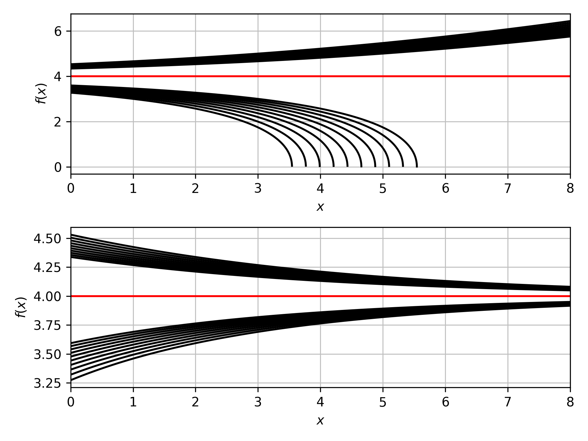

These plots match those in the mathematic notebook exactly. I then moved on to solving the time dependent equation:

\[\frac{\mathrm{d}r}{\mathrm{d}t}=\pm\left(1-\frac{2(m_0^3-t)^{\frac{1}{3}}}{r}\right)\]

This cannot be analytically solved, and so it must be solved using a power series, doing so gives the following plots:

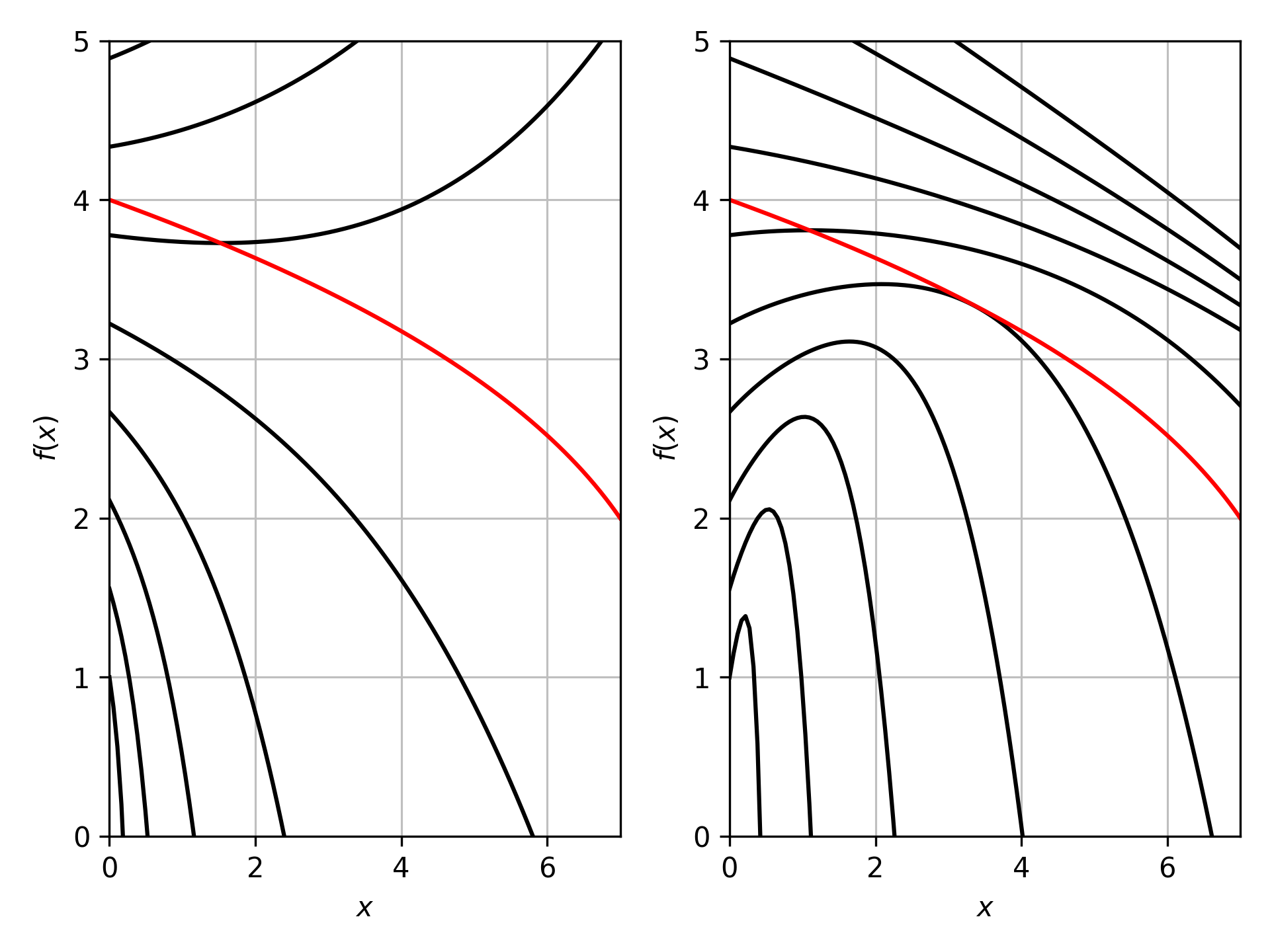
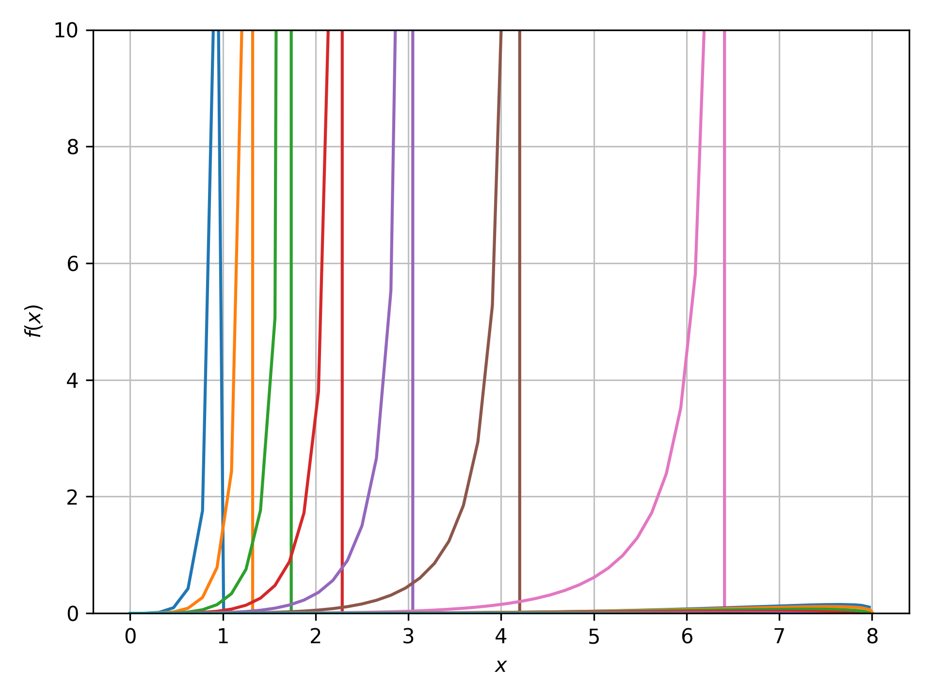
These plots look really encouraging, again they match those in the mathematica notebook. However, there is one feature one would expect to see in any plot in Schwarzschild coordinates, no lines should cross the event horizon as it is a coordinate singularity, but these trajectories cross very easily! This is ultimately an issue with using a power series. Substituting the solutions into the original differential equation should give 0 for an exact solution. However the power series are not exact so we can substitute them in and look at the value at various times and starting conditions to see something analogous to the error:

A better choice of coordinates should be made to calculate these trajectories, taking them from Schwarzschild and mapping to Kruskal coordinates is clearly not a good option. Gullstrand–Painlevé coordinates would be one option, these remove the singularity at the event horizon by replacing the time coordinate with that of an observer falling from infinity with zero initial velocity. This makes them a little harder to interpret, however.